Finding Rhythm in the Latent Space
Building a music generation model from scratch — and listening to what comes out along the way.
Finding Rhythm in the Latent Space
Building a music generation model from scratch — and listening to what comes out along the way.
Attribution
The original audio samples in this post come from my personal music library. All original works belong to their respective artists, songwriters, and rights holders. They are used here solely for research and demonstration.
What I’m trying to do
I set out to build a music generation model that could produce something I would actually want to listen to — not the generic, cliché, slightly-cheesy jingles that many generative audio models default to, but music with the depth, texture, and a likeness to my favorite genres of music. That meant training on my own music library and listening history.
However, this project is about more than generative music. It is really about modelling extremely complex, nuanced and high dimensional time series data. Music happens to be an ideal candidate for this, as it is very easy for humans to interpret.
How the model is steered — what metadata it conditions on, what representation it predicts, how long a context window it sees — changed substantially from version to version and this is detailed in my findings below. At a high level, each training example is a slice of audio split into a context chunk (what came before) and a predict chunk (what the model generated next). Generated spectrograms are turned back into waveform through an open-source log-spectrogram vocoder.
I’ve iterated through eleven versions. The sections below include spectrograms and audio so you can hear how the outputs evolved.
In short: v1 collapses to a smooth, blurry average and sounds like heavily low-passed noise. v3 recovers visible beat structure and rhythmic energy, but timbre is still synth-like. v4 drops the MFCC detour and predicts log-spectrograms directly, but outputs sound like many songs superimposed at once. v5 fixes that collapse — clear rhythm, continuation from context, real spectral structure. The remaining problem is quality drift over time within each segment. v6 tried to fix that drift and stepped backward in quality relative to v5. v7 recovers by warm-starting from v5 and only then adding the autoregressive losses. v8 is the crispest checkpoint yet, at epoch 5, and further training on that stack does not beat it. v9 scales the critics and stays stable without a clear listening win. v10 is the first model that clearly passes v8 epoch 5. v11 keeps training from there on two matched branches: flow-only sounds better on most clips, and the full objective still wins where vocals and punch matter.
Setup
Conditioning: artist label, playlist label, relative position within the track, and a trained embedding of the preceding context audio.
Representations: early versions predict MFCCs (a compact spectral summary); later versions predict log-spectrograms directly and feed them to the vocoder.
v1: conditional VAE on MFCCs
The first attempt is a conditional variational autoencoder on MFCC windows — chosen deliberately for a small model footprint and fast training time as much as for simplicity. It trains stably, but the outputs collapse toward the conditional mean: MFCC heatmaps look washed out and the audio sounds like noise filtered to roughly the right spectral tilt. I also tried a post-trained diffusion model on top of the CVAE output to bring out richer features from those washed-out MFCCs — it recovers a little texture (see the bottom row below), but not enough to cross into music.
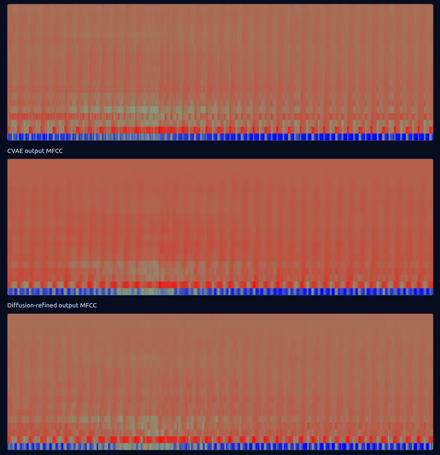
Takeaway: the VAE ignores its latent code and outputs a smoothed average. The loss and architecture both encourage blur. Time to try a different generative objective.
v2: cross-entropy on binned MFCCs
v2 keeps the v1 encoder and the same upsampling decoder. The reconstruction loss is what changes. Standardized MFCC values are clipped to the range −8 to 8 and split into 256 bins, and the last layer is trained with cross-entropy against those bins. v1’s binary cross-entropy on a sigmoid-squashed target could lower the loss by sitting between neighboring values, which is the washed-out conditional mean. A small total-variation penalty on the softmax (weight 0.01) keeps those class probabilities smooth across time, while the chosen bin can still jump.
The MFCC plots pick up a little texture. The audio still sounds like v1, and the model still leans on the artist and playlist conditioning. The encoder bottleneck and the interpolated decoder were smearing time either way, so this stayed a loss experiment — no samples worth posting. That pushed me toward a diffusion-style transformer next.
v3: flow-matching transformer on MFCCs
v3 replaces the VAE with a diffusion transformer trained via flow matching, conditioned on the context MFCC. This is the first version where beats and onsets show up in the output — the MFCC coefficients show visible temporal structure (still noisy, but a clear step up from v1) and the audio has rhythmic energy. A light denoising pass on the MFCC plane cleans up high-frequency speckle without flattening the rhythm.
The timbre is still wrong (noisy synth pad, not the conditioning artist), and the model only generates a few seconds at a time with no autoregressive stitching yet.
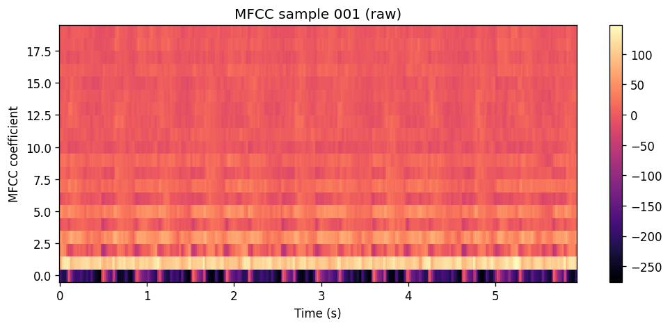
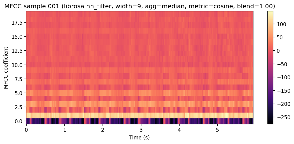
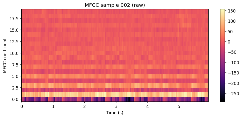
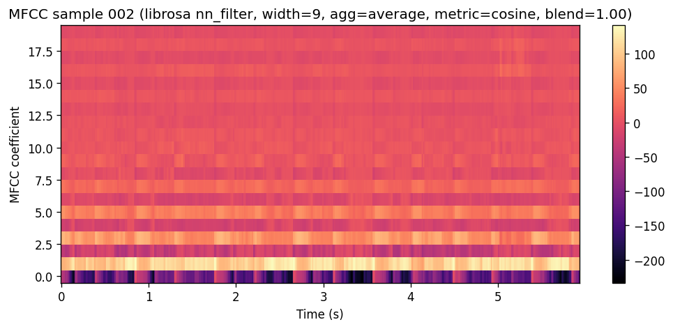
Takeaway: flow matching gives the model a reason to use context — rhythm is real now. But the MFCC → vocoder chain is lossy, and timbre doesn’t land. Next step: predict log-spectrograms directly.
v4: log-spectrogram transformer
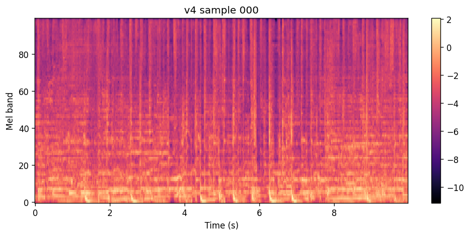
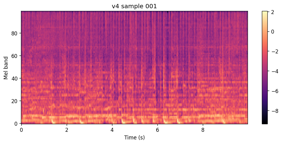
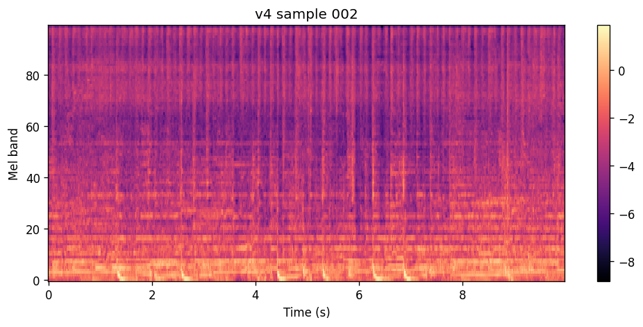
v4 keeps the same flow-matching transformer backbone but predicts log-spectrograms directly instead of MFCCs. The inference chain shrinks to model → log-spectrogram → vocoder. Context windows grow much longer, and the model gets a learned embedding per track on top of artist, playlist, and relative track time conditioning.
Early samples still sound like many songs clashing at once — energy spread uniformly across the spectrogram rather than concentrating into instruments or beats. Same failure mode as v1, different representation: the model is outputting the mean of the training distribution. Pure regression loss encourages blur; it needs a sharpening signal or much more training.
v5: GAN-sharpened log-spectrogram model
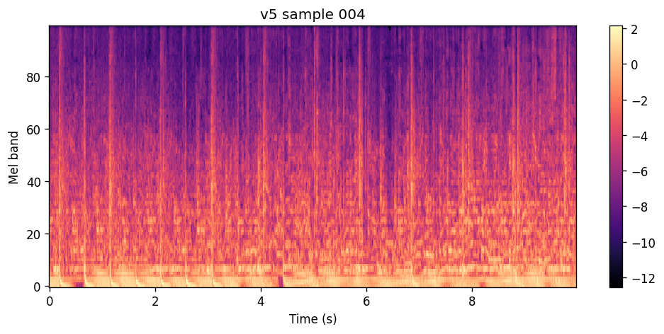
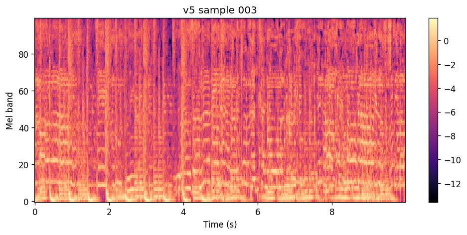
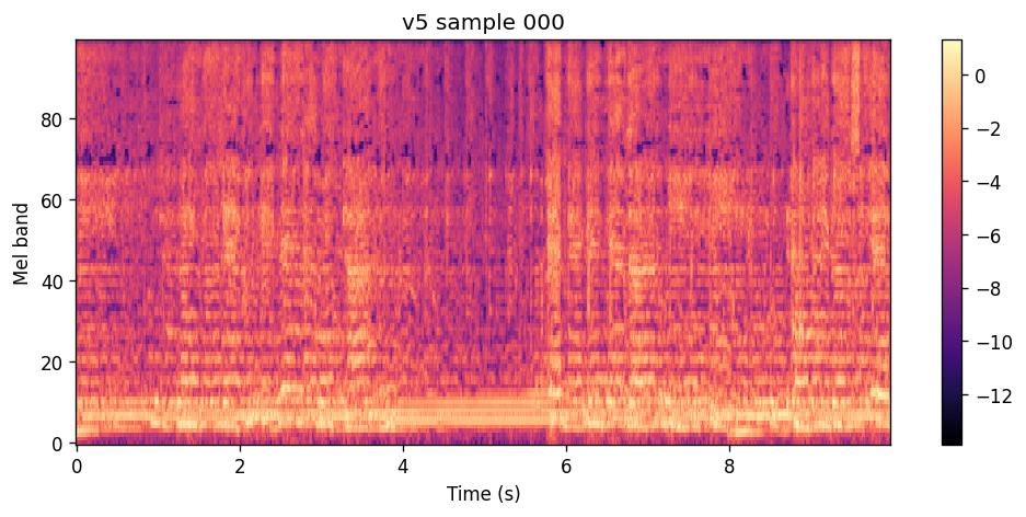
v5 adds an adversarial discriminator on top of the v4 generator. The motivation: regression loss rewards blurry averages; a critic penalizes them. Warm-started from v4, the generator keeps flow-matching for sampling while the GAN pushes outputs toward realistic spectrograms.
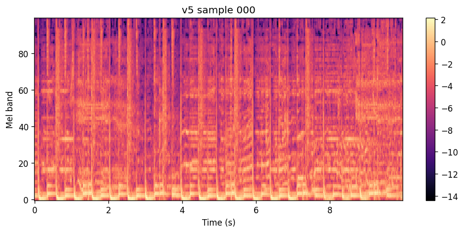
This is the qualitative leap. The superimposed-soup problem is largely gone: clear rhythm, continuation from the context clip, and enough spectral structure that the outputs start to resemble music. Log-spectrogram energy concentrates into formant bands and beat-like striations.
The remaining failure mode is temporal drift within each predict window — the opening sounds coherent, but quality falls off toward the end of the predict window. My hypothesis is error propagation: small per-frame mistakes during flow sampling accumulate, and autoregressive chaining would compound them further.
v6: shorter windows, autoregressive training, cloud GPUs
v6 targets the temporal drift problem from v5. The predict window shrinks from 10 s to 4 s, and training adds scheduled sampling (sometimes feeding the model its own output as context) plus a consistency loss across adjacent windows. At inference, optional overlap-add and classifier-free guidance are available — none of them rescued quality on this run.
Hardware
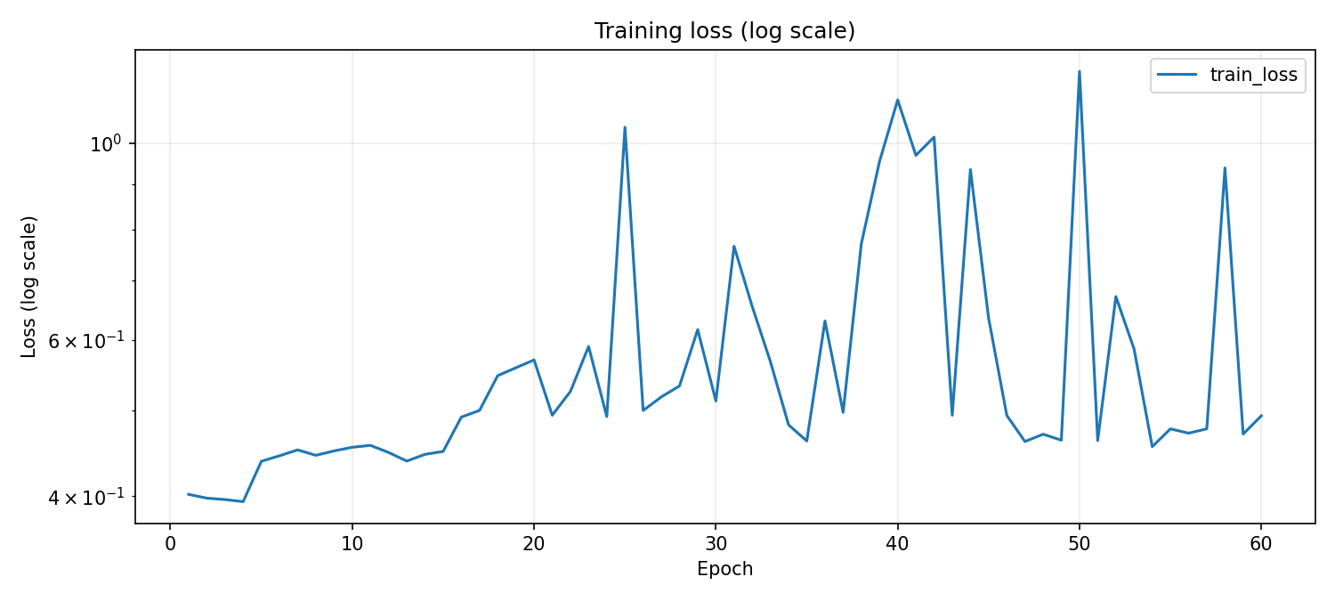
This was the first version trained on cloud GPUs. The idea was purely about iteration speed: use a large effective batch size and distributed training to cover ground quickly and approach the global minimum, then finish locally at batch size 1 on an RTX 5090 in the hope that smaller batches would recover sharper features. Epochs 0–55 ran on a 4× RTX PRO 6000 cluster (effective batch size 24), averaging roughly 180 s per epoch; epochs 56–90 resumed on the 5090. It did not work as expected — training looked unstable after the hardware switch, with a visible discontinuity in the loss curves. That may be partly the batch-size handoff itself, but v6 also introduced enough other changes (shorter predict windows, scheduled sampling, consistency loss) that pinning the regression on any one factor is hard.
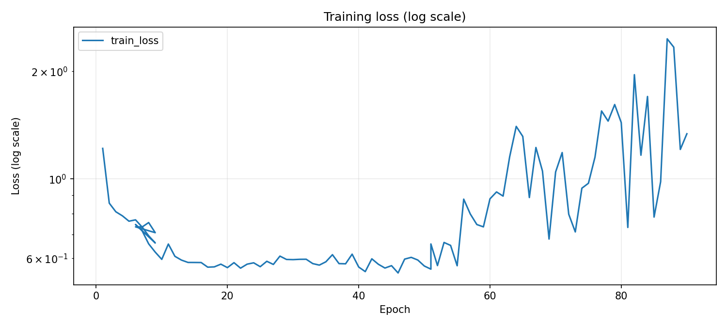
v6 is a regression relative to v5. Audio sounds like many tracks clashing together again — the same failure mode v4 had before GAN sharpening. Rhythm and continuation are weak. Inference is also too slow for real-time use: generating one 4 s clip on the 5090 takes longer than 4 s of wall time.
Samples 1, 3, 4, and 5 below use the same conditioning tracks as the v5 clips for direct comparison.
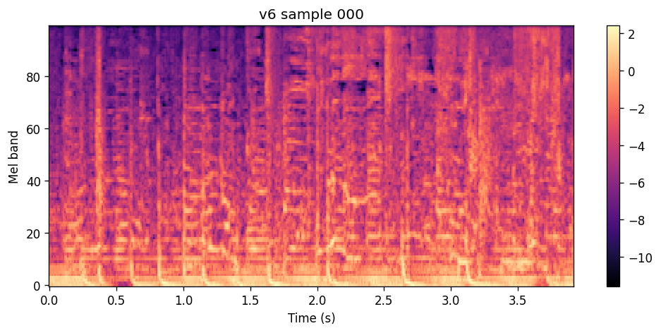
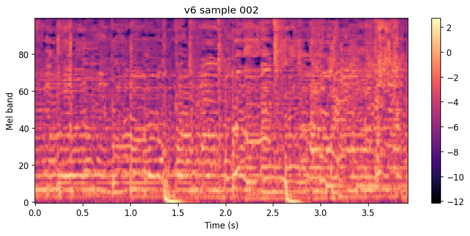
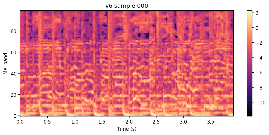
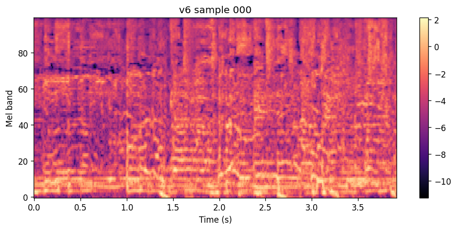
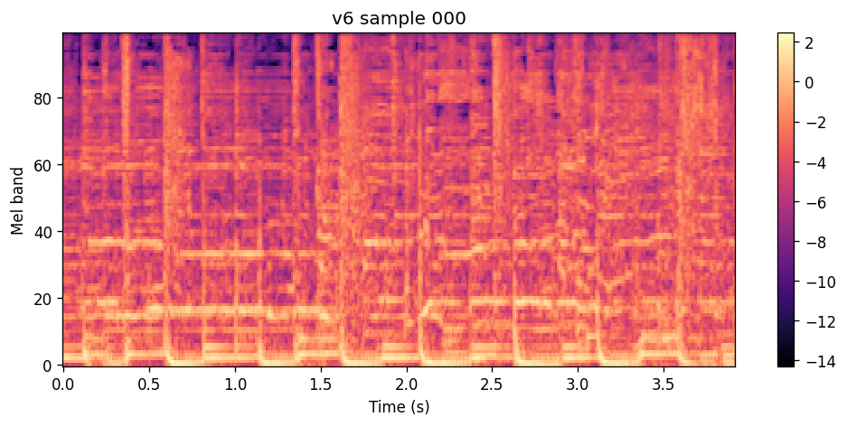
Likely causes: the new training objectives may have pulled the generator back toward averaged predictions, working against the GAN sharpening that fixed v4. The predict head trained from scratch while those objectives were already active. And resuming mid-run on different hardware left a scar in the metrics.
Even so, v6 was a useful ablation rather than a dead end. It taught me a lot about what the data actually demands from the training objective — which losses cooperate with GAN sharpening and which ones quietly push back toward the mean, how sensitive the generator is to batch size and hardware continuity, and how far scheduled sampling and consistency terms can be pushed before they start fighting the core generation task. The audio regressed, but the experiment clarified what v7 needs to do differently.
v7: warm-start from v5, then add the autoregressive losses
v7 is the experiment the v6 failure pointed at. Keep v5’s setup — 60 s of context, a 10 s prediction, the same generator — warm-start from a trained v5 checkpoint, and only later turn on the scheduled sampling and consistency loss that hurt v6 when they were already active. The guess was that v6 regressed because it trained a new, shorter prediction head while those losses were already pulling outputs back toward an average.
Training runs in three phases. The first few epochs refine the flow loss alone. Then the adversarial critic sharpens texture, the same job it did in v5. Only after that, around epoch 15, do scheduled sampling and the consistency loss turn on. Scheduled sampling ramps until the model is often training on its own imperfect context. Context attention is also causal now, so training matches the left-to-right way inference actually extends a clip.
I stopped at epoch 65 on purpose. The loss curves are noisy and do not pick a winner — flow loss bounces as scheduled sampling ramps. Listening does. Before the ramp, texture and the faint vocals are strongest. As the model sees more of its own context, the tail of each window corrupts less, which is what you want for multi-step rollouts, and overall fidelity dips a little. Epoch 65 felt like the balance. Pushing scheduled sampling further did not seem worth it on this pipeline.
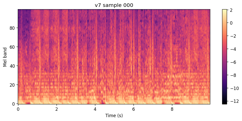
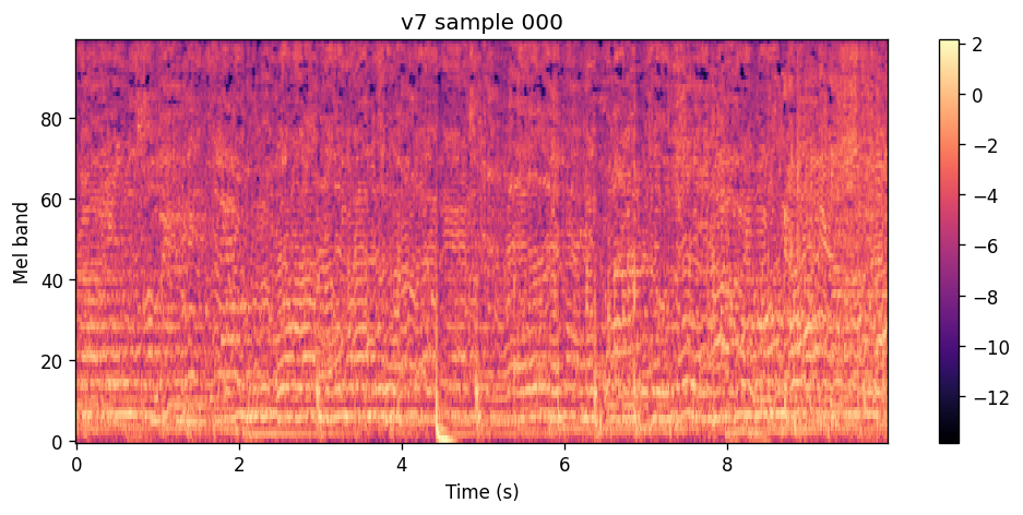
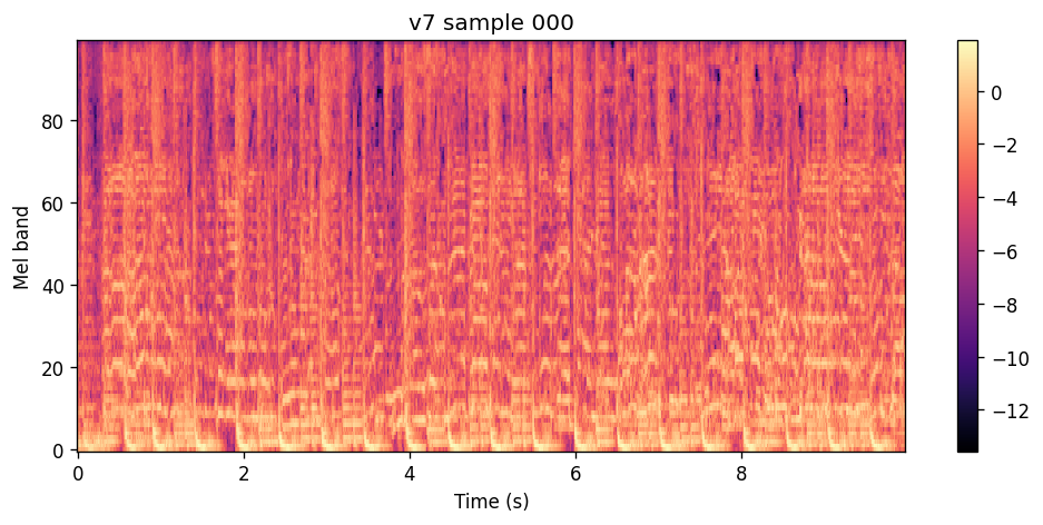
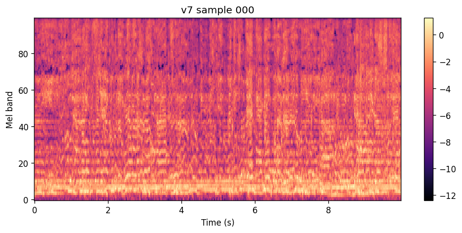
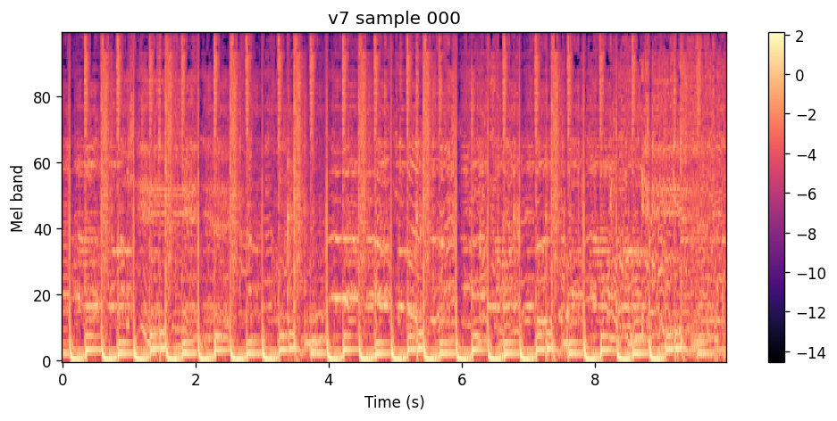
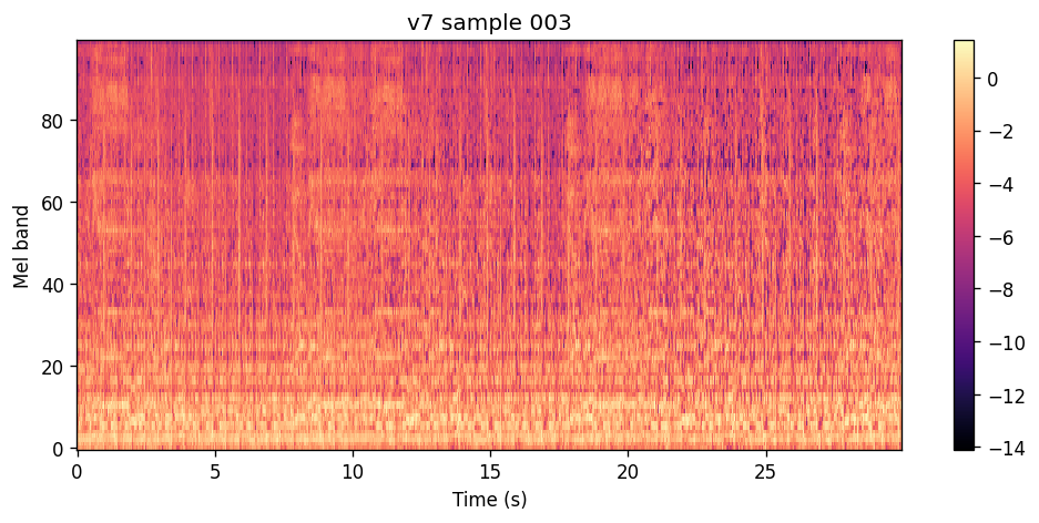
v7 is ahead of v5, and the gap is widest once generation runs for more than one window. The back half of each 10 s segment holds together: sharper transients, less harmonic smear, percussion that stays crisp at higher tempos, and the first faint vocals. The v6 losses were usable. The order was the part that mattered. v7 inherits a generator that already knows how to be sharp, then teaches it to survive its own mistakes.
Samples below are one 10 s generation from 60 s of context, on the same crops as v5 and v6.
v8: a second critic for the whole segment
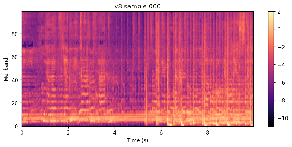
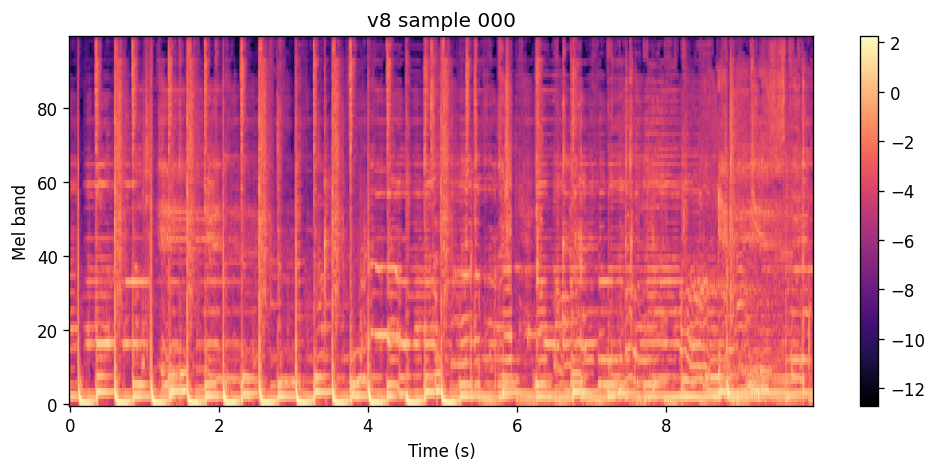
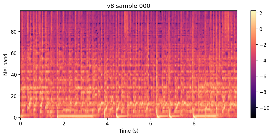
v7’s critic is good at local spectrogram texture and silent on whether ten seconds hangs together as music. v8 keeps the v7 generator and adds a second critic that scores only the predicted 10 s. It asks whether that segment unfolds like real music for the artist and playlist, including harder negatives drawn from the same playlist, and it sees frozen context from the generator so it can judge a continuation. The local critic stays. Flow matching stays the anchor. The new term is supposed to ramp in slowly.
The first run did the opposite. Warm-started from v7 epoch 65, it sounded good at epoch 5 and had fallen into low-frequency soup by epochs 9–15, once the new critic pushed hard and the flow loss climbed. That set the rule for the rest of v8: the segment-level signal ramps gently, and flow stays dominant.
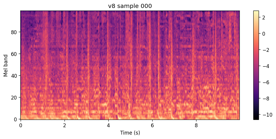
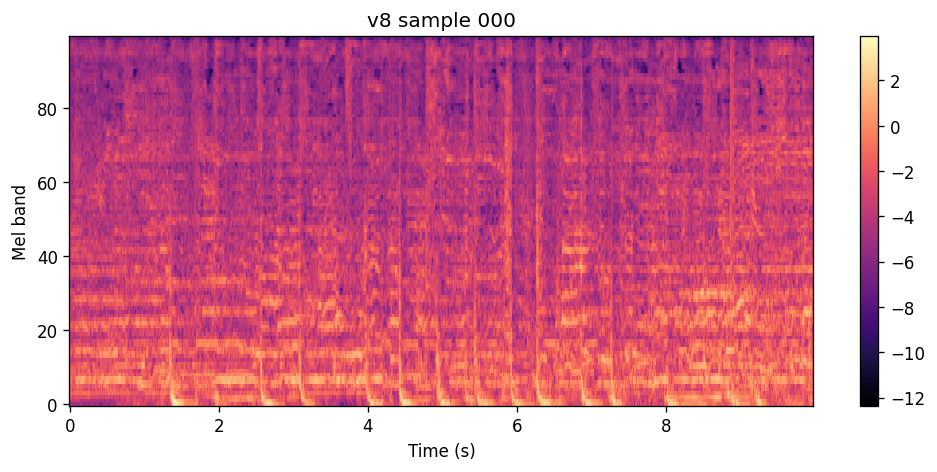
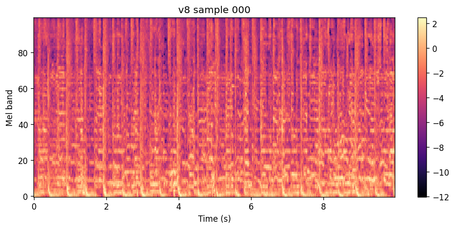
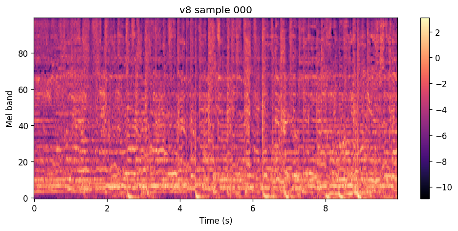
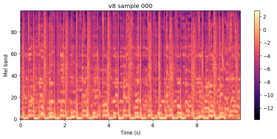
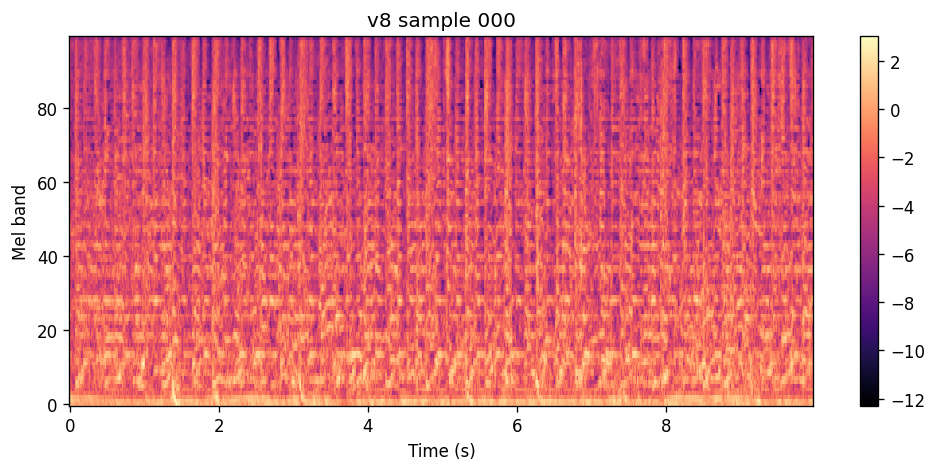
Epoch 5 is the best v8 checkpoint, and the crispest audio in the project up to this point. Transients are clear, rhythm holds, and vocals are actually noticeable on some clips. Later checkpoints on this stack either dulled the texture or optimized an objective that did not pay off in headphones.
Dropping the local critic, to see if the new one could carry sharpening alone, sent outputs back to soup. Both critics are required. A longer run with the ramp fixed stayed stable for dozens of epochs and coped better when the conditioning changed — the model was learning plausible 10 s segments, which is what you want for generalization, and those segments diverge from the exact recording at the window tails. Multi-step rollouts still had an audible seam at the overlap. Turning the consistency loss up to force the overlaps to match made the seam worse. I reverted that fine-tuning. Epoch 5 stays the checkpoint I actually use.
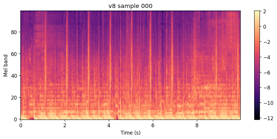
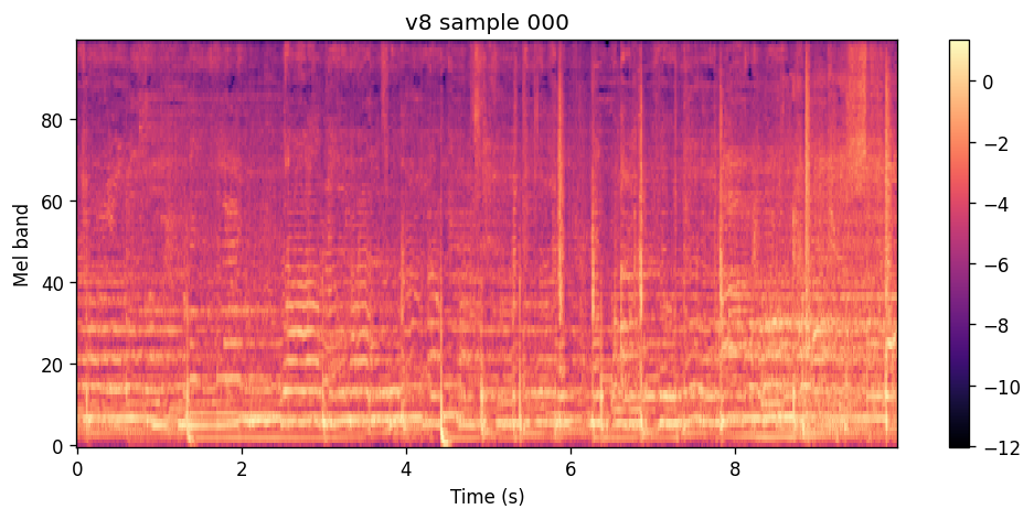
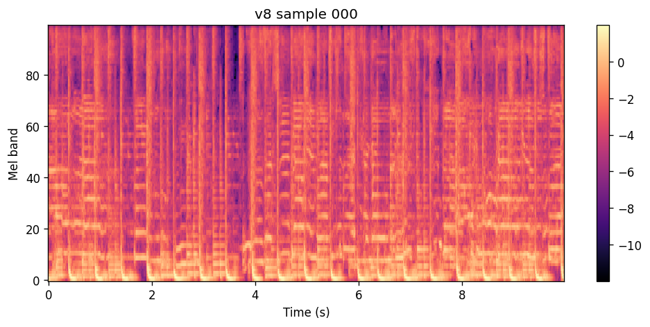
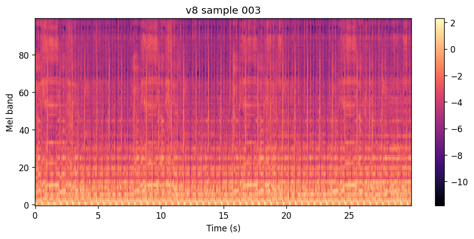
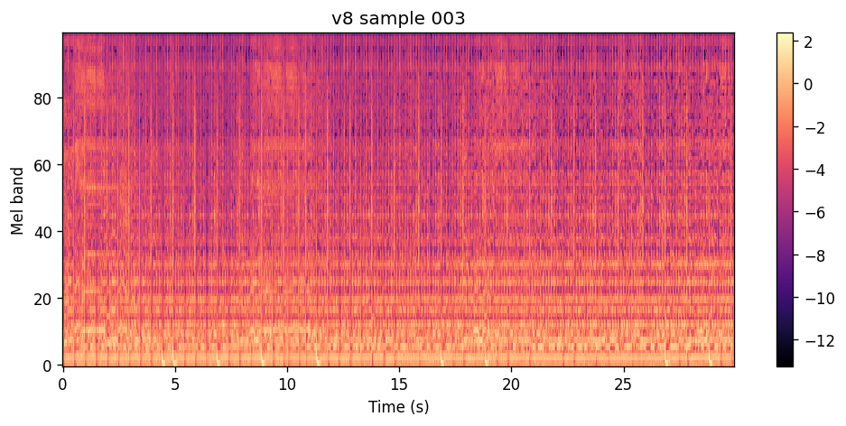
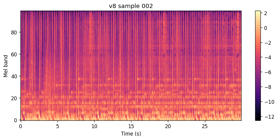
The segment critic still earned its place. Once the schedule was fixed, joint training stayed stable, and the model coped better with condition changes. The cost is that “plausible music” and “this exact recording” pull in different directions, which is why the overlap penalty backfired. The critic itself was also small next to the generator, which is what v9 tried to fix.
v9: bigger critics on the epoch 5 generator
v9 keeps the v8 epoch 5 generator and rebuilds both critics much larger: the local critic from about 2 million parameters to about 13 million, the segment critic from about 60 million to about 256 million. The generator architecture does not change. Scheduled sampling is gone — epoch 5 is already realistic enough that training on synthetic context gives up sharpness for tail robustness, and the listening tests did not justify it. Overlap consistency is replaced by a narrower term. Only the opening frames of the prediction, right where generation meets the real context, are pulled toward the ground-truth spectrogram. That anchors the boundary and leaves the tail alone.
The critics train by themselves for eight epochs with the generator frozen. Joint training starts at epoch 9. Through epoch 18 the new critic judges samples and does not yet push the generator, and that checkpoint still sounds like v8 epoch 5. From epoch 19 its pressure on the generator ramps, and by epoch 33 it is meant to outweigh the local critic. The leading-edge consistency term turns on at epoch 34. The clips below are epoch 40.
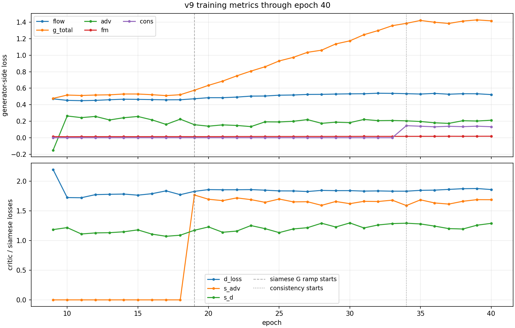
Epoch 18 is still the v9 listening reference. Epoch 40 is stable, and it is a serious competitor to v8 epoch 5 rather than a replacement. Loss stays numerically stable through epoch 40, and the samples do not sound better than epoch 18. Failure modes are the ones a segment-level critic invites: sharp elements that clash instead of grooving, or energy that washes out as the model matches “music like this” instead of this recording. Leading-edge consistency, at least, turns on without the immediate regression of v8’s overlap fine-tuning. Bigger critics can be trained on this generator. Stronger pressure from them still has to be checked by ear, and on that check v9 does not move the project forward.
v10: a larger model, the v7 recipe, and spectrogram detail
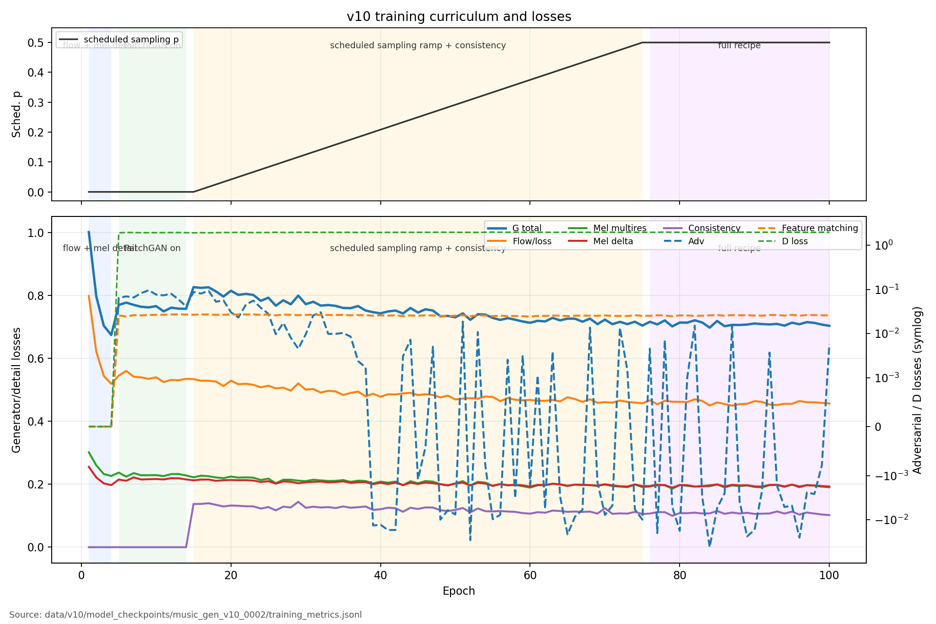
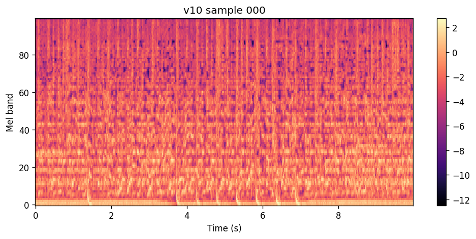
After two versions of critic experiments, I went back to the simpler v7 line and changed the things that had actually moved the audio: scale, and a direct penalty on spectrogram detail. v10 trains a larger generator from scratch. Alongside flow matching it matches the log-spectrogram at several time resolutions and matches how energy changes from frame to frame, so contours are supervised directly. The curriculum is the v7 one. Flow and detail first, then the adversarial critic, then scheduled sampling and leading-edge consistency, through a full 100 epochs. This was the first uninterrupted run on larger hardware — two H100s — with comparison samples saved along the way.
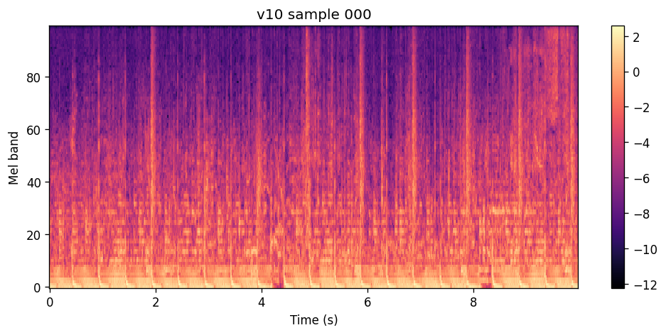
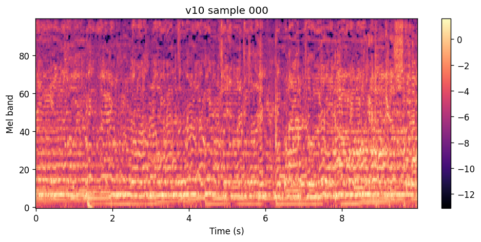
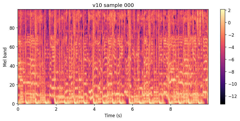
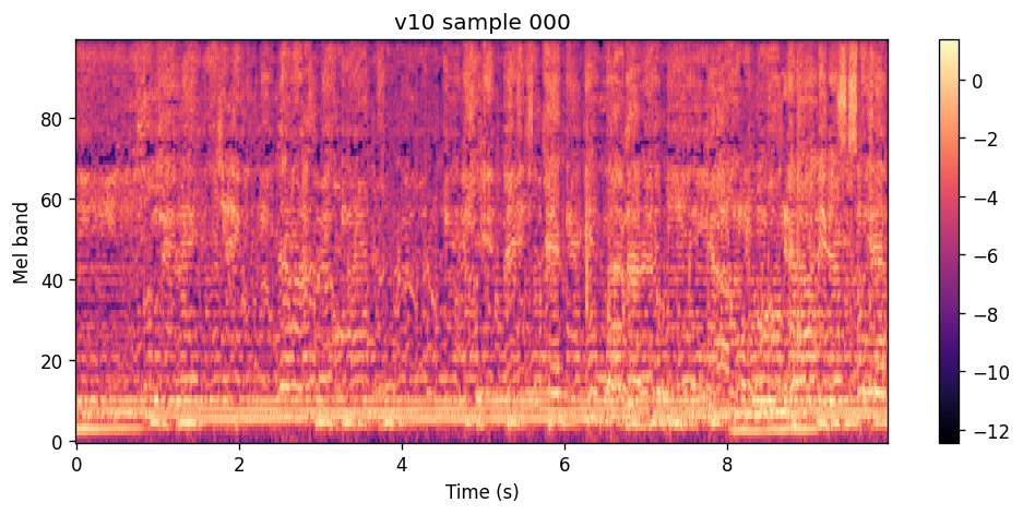
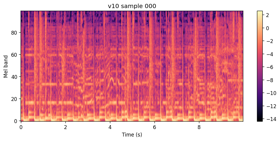
Early epochs show structure in the spectrogram and still sound washed out: parts clash, and there is no heavy beat. Around epoch 20, listening is rougher even as the spectrograms get busier. Vocal-like artifacts appear before convincing beats and drums. By epoch 50 there are occasional beats and sharper transients, and a clip more often sounds like one track, but the texture is scrubbed and distorted, the low end is weak, and vocals are not really there. Epoch 66 is a bit better, with the same failure modes.
Epoch 100 is the new best. Against v8 epoch 5 it has more complex patterns, more coherent structure, less distortion, and audible vocal snippets. It is unfinished: jitter is still obvious, and it wants another training pass. Sampling uses classifier-free guidance; these clips use a guidance scale of 1.5. Scaling the model and adding the detail losses moved the audio. Scaling the critics had not.
v11: keep training, on two recipes
v11 starts from the v10 epoch 100 checkpoint and asks whether another 40 epochs of the same recipe cleans up the remaining artifacts. Two branches share that initialization and both run through epoch 140. The full-objective branch keeps the whole v10 recipe: flow, the adversarial critic, feature matching, the spectrogram-detail losses, leading-edge consistency, and scheduled sampling. The flow-only branch keeps velocity matching and turns the rest off.
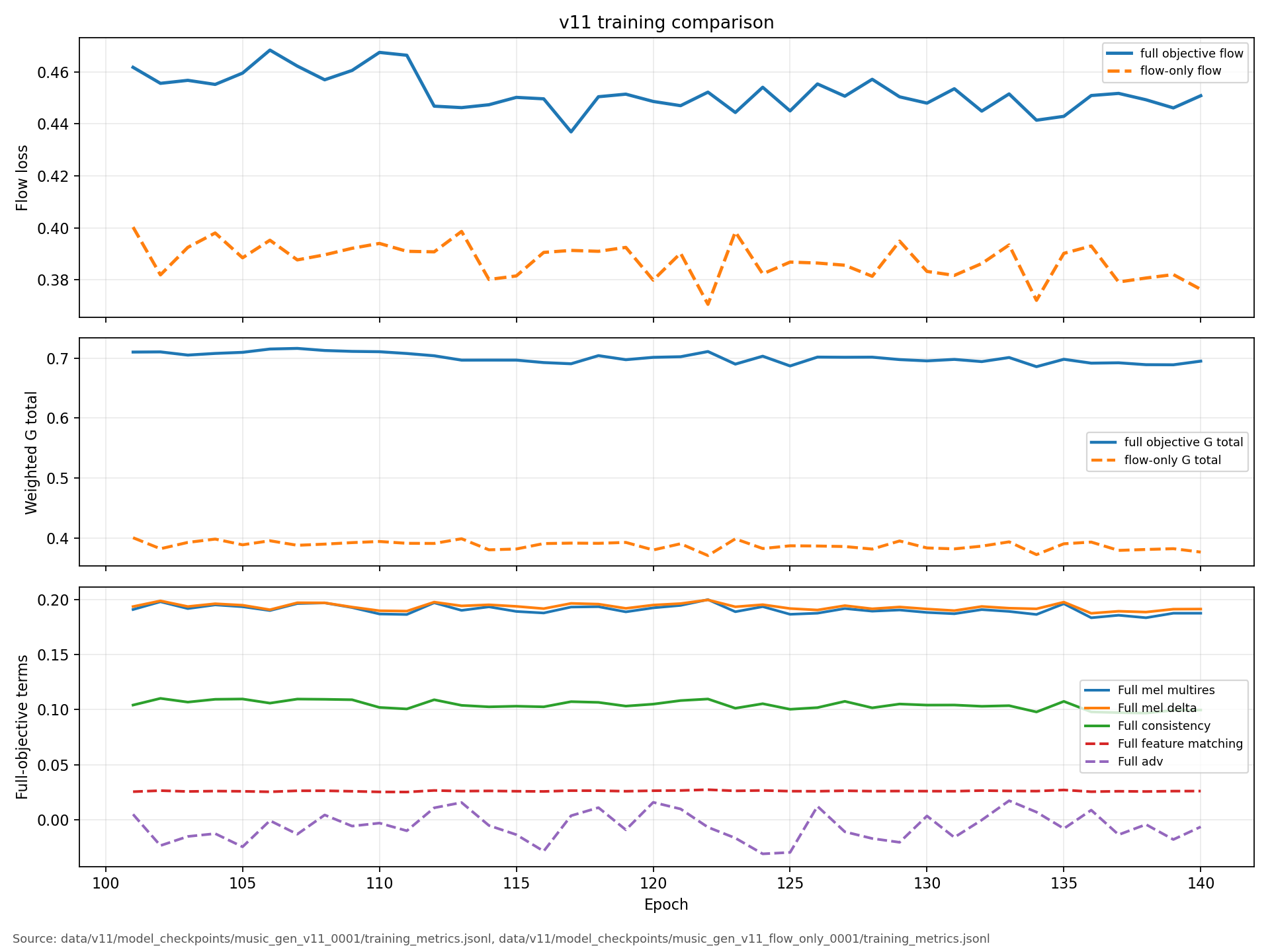
Flow-only sounds better on most clips. The full objective still wins where vocal identity and punch matter. On the Purple Disco Machine crop below, the full-objective branch tracks the vocal and the source more closely, with more grit. Flow-only is cleaner there, and less faithful.
Flow-only pulls ahead on robustness. Error builds more slowly across autoregressive steps, and a segment that has drifted can come back. It is also the first branch with something like song-scale shape: in one three-step rollout the beat drops out, the intensity falls, and then the track starts building again.
That split is the result of this run. The full objective keeps training from collapsing and pushes the model to learn detail, and it leaves sampling artifacts. Flow-only is the refinement pass.
The first carousel is the six fixed 10 s crops, both branches, guidance 1.5. Each slide has the full objective first and flow-only second. The second carousel is three-step rollouts, about 30 s: Stromae, where flow-only limits error across the steps, then two flow-only clips where a noisy opening recovers and a phrase actually builds.
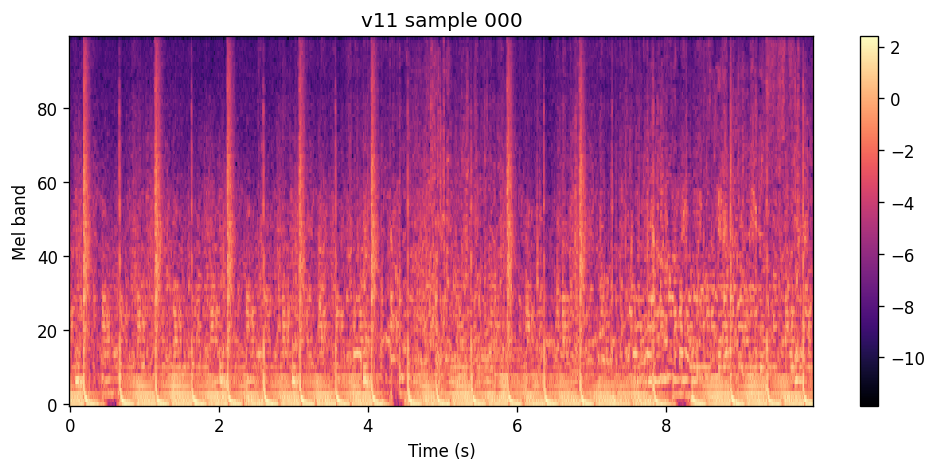
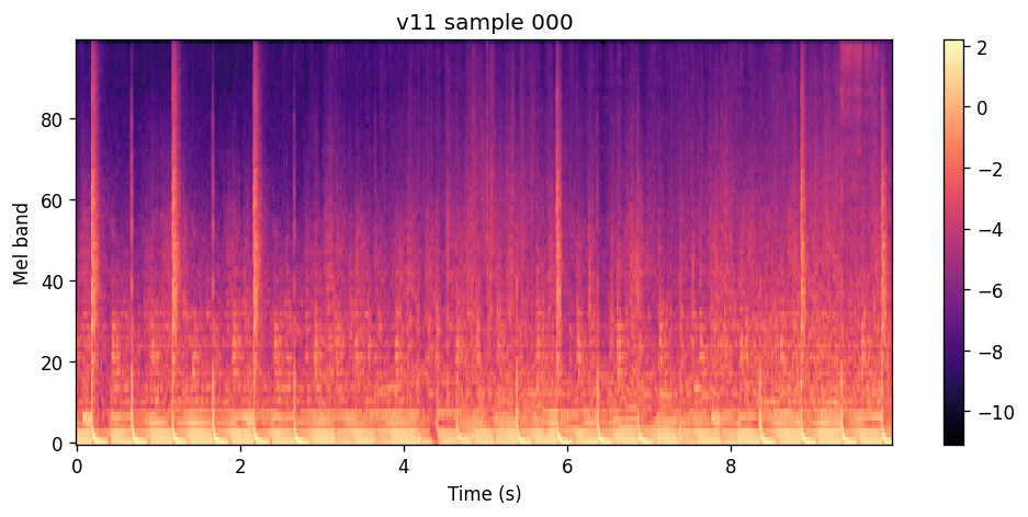
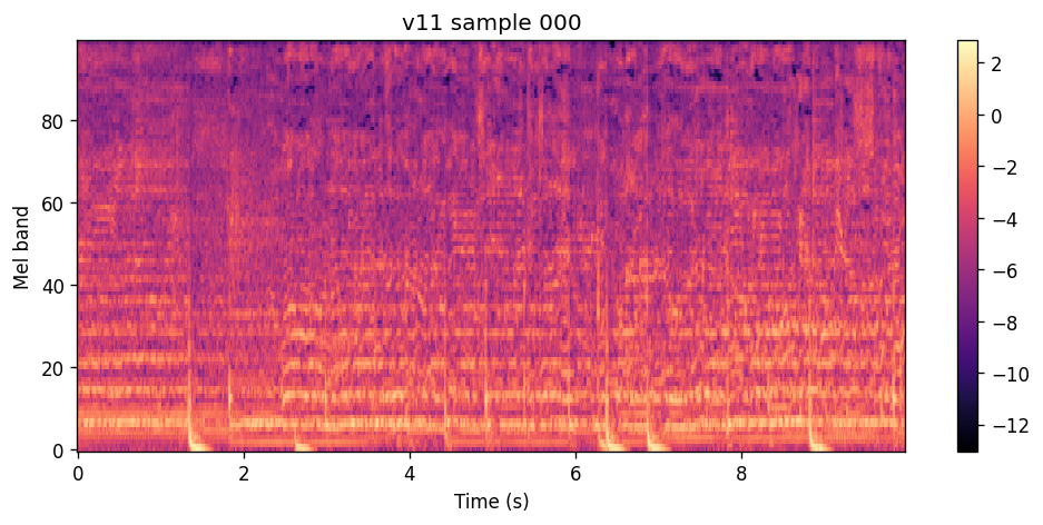
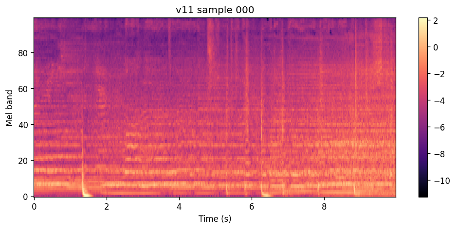
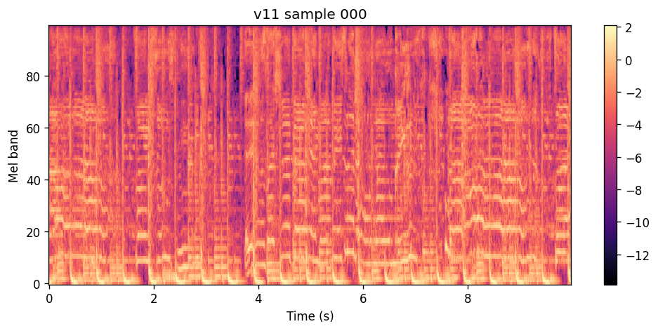
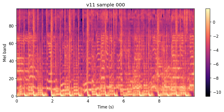
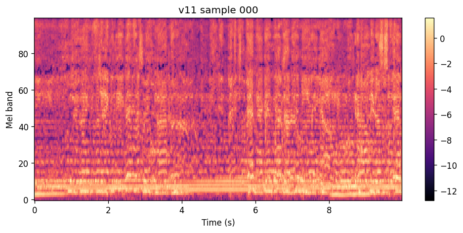
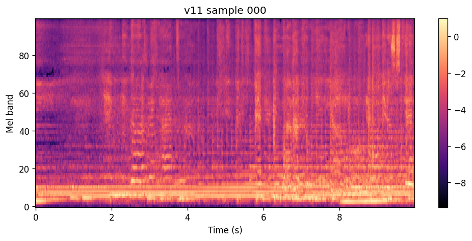
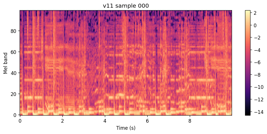
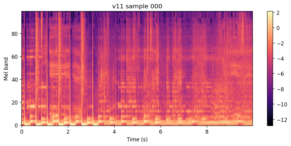
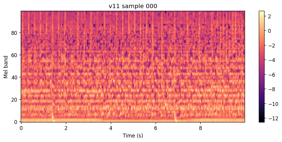
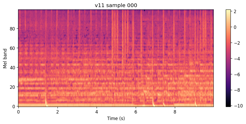
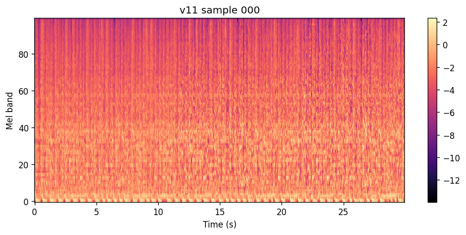
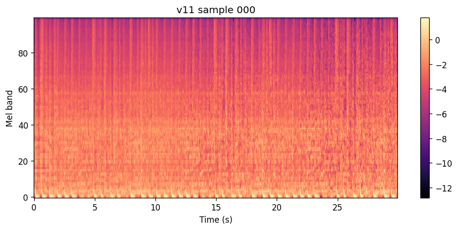
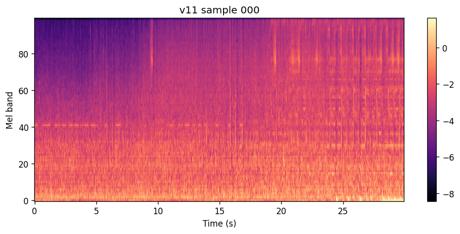
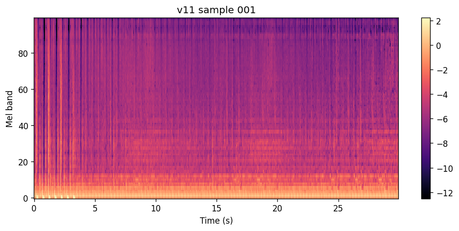
v10 epoch 100 was the first time the project clearly passed its old listening peak. v11 shows what that peak still needs: flow-only holds a rollout together, and the full objective is what keeps the detail and the vocal punch from washing out.
What I learned about modeling high-dimensional time-series data
I spent most of this project watching the loss function go down and then pressing play and disagreeing with it. That is counterintuitive — a decreasing loss is supposed to mean the model is getting better — but this kept happening. The clip would turn to soup, or a critic would settle for “a song like this” instead of the song I conditioned on. The changes that actually improved the model were the ones aimed at something I could hear: the texture up close, the shape of a phrase, whether the next moment follows from this one. I am confident that I could achieve much better results with longer training runs and a larger model, but this starts to enter the realm of unjustified compute expense. For what I set out to achieve I am plenty happy and have learnt a lot along this journey.
Music is complex, structured, nuanced, and it is art - hence, the qualitative analysis outweighed the loss numbers. I will conclude on a more philosophical note: Even if I were able to perfectly model my taste in music and fool my ear, I wouldn’t consider it art. It would eventually become boring as it is stuck in time, and is simply interpolating between a fixed domain. Music is an art form and this is something that requires a human, it requires feelings, emotions, human context and purpose - things that could never be accomplished by a machine. We should never stop creating and enjoying art.